Table of Contents
- What You Will Learn
- Understanding Multiple Linear Regression
- The Student Performance Dataset
- Building Your Model Step by Step
- Validating Your Results
- Key Takeaways
What You Will Learn
In this tutorial, you will discover how to build a multiple linear regression model completely from scratch. By the end, you will understand not just how to use machine learning, but how it actually works under the hood. This knowledge will set you apart from developers who only know how to import libraries.
Why Build From Scratch?
Building models from scratch provides three key advantages:
- Deep Understanding: You learn the mathematics behind the algorithms
- Better Debugging: When things go wrong, you know exactly where to look
- Interview Readiness: Top companies often ask candidates to implement algorithms from scratch
Let me guide you through building a model that predicts student performance with remarkable accuracy.
Understanding Multiple Linear Regression
Before diving into code, let us establish a solid foundation. Multiple linear regression finds the best-fitting line (or hyperplane) through multi-dimensional data. Think of it as drawing the most accurate trend line possible through a cloud of data points.
The mathematical formula at the heart of our model is:
y = β₀ + β₁x₁ + β₂x₂ + ... + βₙxₙ
Where:
- y represents what we want to predict (student performance)
- β values are coefficients showing how much each factor matters
- x values are our input features (study hours, previous scores, etc.)
The Normal Equation: Your Secret Weapon
Instead of using iterative methods like gradient descent, we will use the normal equation for an elegant, one-shot solution:
β = (X^T × X)^(-1) × X^T × y
This equation finds the optimal coefficients instantly. No loops. No iterations. Just pure mathematical precision.
The Student Performance Dataset
Our journey begins with real data from Kaggle containing information about 1,000 students. Each row tells a story about a student's habits and their resulting academic performance.
The dataset includes six columns:
- Hours Studied: Daily study time (1-10 hours)
- Previous Scores: Historical performance (0-100)
- Extracurricular Activities: Yes/No participation
- Sleep Hours: Nightly rest (4-10 hours)
- Sample Question Papers Practiced: Exam preparation (0-10)
- Performance Index: Our target variable (0-100)
You can access the complete implementation and dataset here: Kaggle Notebook - Multi Linear Regression From Scratch
Building Your Model Step by Step
Step 1: Data Exploration and Feature Selection
The first rule of machine learning is to understand your data before touching any algorithms. Let us start by examining which factors actually influence student performance.
import numpy as np
import pandas as pd
import matplotlib.pyplot as plt
import seaborn as sns
from scipy import stats

# Load the dataset
data_df = pd.read_csv("Student_Performance.csv")

# Convert categorical data to numerical
data_df['Extracurricular Activities'] = data_df['Extracurricular Activities'].map({'Yes':1, 'No':0})

# Calculate correlations with our target variable
corr_m = data_df.corr()
print(corr_m['Performance Index'])
The correlation analysis reveals fascinating insights:
- Previous Scores (0.92): Nearly perfect correlation - past performance strongly predicts future success
- Hours Studied (0.37): Moderate impact - effort matters, but it is not everything
- Extracurricular Activities (0.02): Surprisingly minimal impact
- Sleep Hours (0.05): Low correlation, but we will keep it to capture potential hidden patterns
Based on this analysis, we select three features for our model: Previous Scores, Hours Studied, and Sleep Hours.
Step 2: Data Preprocessing - The Foundation of Success
Clean, well-prepared data is essential for any machine learning model. Our preprocessing function handles three critical tasks:
def data_processing(data_df, features_columns, target_column, train_size=0.8, random_state=42):
    # Select only the features we need
    desired_data = data_df[features_columns + [target_column]].copy()

    # Shuffle to ensure random distribution
    shuffle_df = desired_data.sample(frac=1, random_state=random_state).reset_index(drop=True)

    # Split into training and testing sets
    train_sz = int(train_size * len(desired_data))
    train_set = shuffle_df[:train_sz]
    test_set = shuffle_df[train_sz:]

    # Separate features and target
    X_train = train_set[features_columns]
    y_train = train_set[target_column]
    X_test = test_set[features_columns]
    y_test = test_set[target_column]

    # Standardization - bringing all features to the same scale
    train_mean = X_train.mean()
    train_std = X_train.std()
    X_train_std = (X_train - train_mean) / train_std
    X_test_std = (X_test - train_mean) / train_std

    return X_train_std, y_train, X_test_std, y_test
Why Standardization Matters: Without standardization, features with larger scales (like Previous Scores: 0-100) would dominate features with smaller scales (like Hours Studied: 1-10). Standardization ensures every feature competes fairly.
Step 3: Implementing the Learning Algorithm
Now comes the exciting part - implementing the actual learning algorithm. This is where mathematical theory transforms into working code:
def train_and_eval_model(X_train, y_train, X_test, y_test, plot_residuals=True):
    # Add intercept column (for the β₀ term)
    n_train = X_train.shape[0]
    n_test = X_test.shape[0]
    X_train_intercept = np.column_stack([np.ones(n_train), X_train])
    X_test_intercept = np.column_stack([np.ones(n_test), X_test])

    # Apply the normal equation
    X_T = X_train_intercept.T
    try:
        # This single line finds the optimal coefficients
        beta = np.linalg.solve(X_T @ X_train_intercept, X_T @ y_train)
    except np.linalg.LinAlgError:
        # Fallback for singular matrices
        beta = np.linalg.lstsq(X_train_intercept, y_train, rcond=None)[0]

    # Generate predictions
    y_train_pred = X_train_intercept @ beta
    y_test_pred = X_test_intercept @ beta

    # Calculate performance metrics
    # ... (metrics calculation code continues)
The beauty of this approach lies in its elegance. While gradient descent would require hundreds of iterations, the normal equation solves everything in one computation.
AdSense Ad Placement - Middle of Article
Step 4: Model Evaluation - Trust but Verify
Building a model is only half the battle. We must rigorously validate its performance:
# Calculate R-squared - how much variance we explain
ss_total = np.sum((y_true - np.mean(y_true)) ** 2)
ss_residual = np.sum((y_true - y_pred) ** 2)
r2 = 1 - (ss_residual / ss_total)

# Calculate RMSE - average prediction error
rmse = np.sqrt(np.mean((y_true - y_pred) ** 2))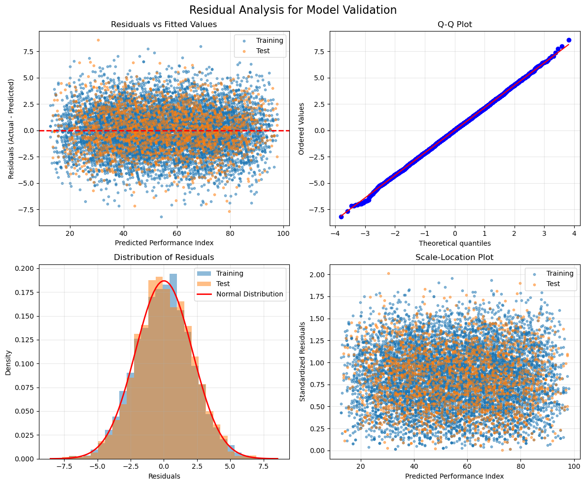
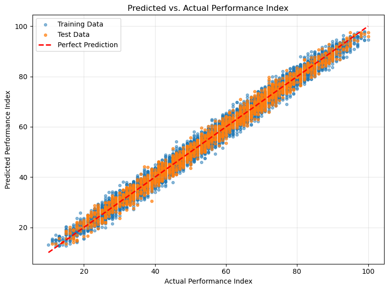
Our model achieves impressive results:
- R² Score: 0.988 (explaining 98.8% of variance)
- RMSE: 2.14 points (on a 0-100 scale)
- No Overfitting: Test performance matches training performance
Validating Your Results
Understanding Residual Plots
Residual plots are like health checkups for your model. Each plot tells a different story:
- Residuals vs Fitted Values: Random scatter confirms no systematic bias
- Q-Q Plot: Points following the line confirm normal distribution
- Histogram: Bell curve shape validates our assumptions
- Scale-Location: Horizontal band shows consistent accuracy
Running the Complete Model
Here is how everything comes together:
import numpy as np
import pandas as pd
import matplotlib.pyplot as plt
import seaborn as sns
from scipy import stats

# First lets import the data
# Note: You will need to change this file path to the location of the dataset on your computer.
data_file = "~/path_to_your_file"

# create a pandas data frame
data_df = pd.read_csv(data_file)

# Lets print the dataset to see how it is structured.
print(data_df.head())

#Remapping "Extracurricular Activities"
data_df['Extracurricular Activities'] = data_df['Extracurricular Activities'].map({'Yes':1, 'No':0})

#Lets separate features from target
features = data_df.iloc[:, :-1]
target   = data_df.iloc[:, -1]

#Lets give each column names
features_names = features.columns.to_list()
target_name    = data_df.columns[-1]

#Time to check correlation
corr_m = data_df.corr()

#lets print values
print(corr_m['Performance Index'])

#lets create a figure for a different visualization
plt.figure(figsize=(8, 6))

# Create heatmap
sns.heatmap(corr_m, annot=True, cmap='coolwarm', center=0, fmt='.2f', square=True, linewidths=0.5, cbar_kws={"shrink": 0.8})
plt.title('Correlation Matrix of Student Performance Features', fontsize=16)
plt.tight_layout()
plt.show()

#lets create a function to preprocess the dataset by normalizing it and splitting into 80% train and 20% test.
def data_processing(data_df, features_columns, target_column, train_size=0.8, random_state=42):

    #make copy of dataframe with the desired features and target
    desired_data = data_df[features_columns + [target_column]].copy()

    #shuffle dataset
    shuffle_df = desired_data.sample(frac = 1, random_state=random_state).reset_index(drop=True)

    #train_set
    train_sz  = int(train_size * len(desired_data))
    train_set = shuffle_df[:train_sz]

    #test_set
    test_set = shuffle_df[train_sz:]

    X_train = train_set[features_columns]
    y_train = train_set[target_column]
    X_test  = test_set[features_columns]
    y_test  = test_set[target_column]

    #apply standardization formula to features
    train_mean  = X_train.mean()
    train_std   = X_train.std()
    X_train_std = (X_train - train_mean) / train_std
    X_test_std  = (X_test - train_mean) / train_std

    return X_train_std, y_train, X_test_std, y_test

def train_and_eval_model(X_train, y_train, X_test, y_test, plot_residuals=True, plot_fit=True):
    # Create a feature matrix with intercept column
    n_train = X_train.shape[0]
    n_test  = X_test.shape[0]
    X_train_intercept = np.column_stack([np.ones(n_train), X_train])
    X_test_intercept  = np.column_stack([np.ones(n_test), X_test])

    # Solve normal equations beta = (X^T * X)^(-1) * X^T * y
    # Help to find the optimal coefficients in one direct computation
    X_T = X_train_intercept.T
    try:
        beta = np.linalg.solve(X_T @ X_train_intercept, X_T @ y_train)
    except np.linalg.LinAlgError:
        beta = np.linalg.lstsq(X_train_intercept, y_train, rcond=None)[0]

    # Generate predictions
    y_train_pred = X_train_intercept @ beta
    y_test_pred = X_test_intercept @ beta

    # Calculate residuals (actual - predicted)
    train_residuals = y_train - y_train_pred
    test_residuals = y_test - y_test_pred

    #Create Linear regression plot
    if plot_fit:
        create_prediction_vs_actual_plot(y_train, y_train_pred, y_test, y_test_pred)

    # Create residual plots
    if plot_residuals:
        create_residual_plots(y_train, y_train_pred, train_residuals,
                              y_test, y_test_pred, test_residuals)

    # Calculate performance metrics
    def compute_metrics(y_true, y_pred, dataset_name):
        # Mean squared error formula
        mse = np.mean((y_true - y_pred) ** 2)
        # Root mean squared error formula
        rmse = np.sqrt(mse)

        # R-squared: proportion of variance explained (1.0 = perfect, 0.0 = no better than mean)
        ss_total = np.sum((y_true - np.mean(y_true)) ** 2)
        ss_residual = np.sum((y_true - y_pred) ** 2)
        r2 = 1 - (ss_residual / ss_total) if ss_total > 0 else 0

        return {
            f'{dataset_name}_mse': mse,
            f'{dataset_name}_rmse': rmse,
            f'{dataset_name}_r2': r2,
            f'{dataset_name}_samples': len(y_true)
        }

    # Compute metrics for both training and test sets
    train_metrics = compute_metrics(y_train, y_train_pred, 'train')
    test_metrics = compute_metrics(y_test, y_test_pred, 'test')

    # Display the metrics
    display_metrics_pandas(train_metrics, test_metrics)

    return {'coefficients': beta, 'train_metrics': train_metrics, 'test_metrics': test_metrics, 'predictions': { 'train': y_train_pred, 'test': y_test_pred},
        'residuals': {'train': train_residuals, 'test': test_residuals}}

def display_metrics_pandas(train_metrics, test_metrics):

    metrics_data = {
        'Training': [
            train_metrics['train_mse'],
            train_metrics['train_rmse'],
            train_metrics['train_r2'],
            train_metrics['train_samples']
        ],
        'Test': [
            test_metrics['test_mse'],
            test_metrics['test_rmse'],
            test_metrics['test_r2'],
            test_metrics['test_samples']
        ]
    }

    df = pd.DataFrame(metrics_data,
                      index=['MSE', 'RMSE', 'R²', 'Samples'])
    for col in df.columns:
        df.loc[['MSE', 'RMSE', 'R²'], col] = df.loc[['MSE', 'RMSE', 'R²'], col].round(4)

    print("\n" + "="*40)
    print("MODEL PERFORMANCE METRICS")
    print("="*40)
    print(df.to_string())
    print("="*40 + "\n")

def create_residual_plots(y_train, y_train_pred, train_residuals, y_test, y_test_pred, test_residuals):

    # Create a figure with 4 subplots
    fig, axes = plt.subplots(2, 2, figsize=(12, 10))
    fig.suptitle('Residual Analysis for Model Validation', fontsize=16)

    # 1. Residuals vs Fitted Values
    ax1 = axes[0, 0]
    ax1.scatter(y_train_pred, train_residuals, alpha=0.5, label='Training', s=10)
    ax1.scatter(y_test_pred, test_residuals, alpha=0.5, label='Test', s=10)
    ax1.axhline(y=0, color='red', linestyle='--', linewidth=2)
    ax1.set_xlabel('Predicted Performance Index')
    ax1.set_ylabel('Residuals (Actual - Predicted)')
    ax1.set_title('Residuals vs Fitted Values')
    ax1.legend()
    ax1.grid(True, alpha=0.3)

    # 2. Q-Q Plot for Normality Check
    ax2 = axes[0, 1]
    all_residuals = np.concatenate([train_residuals, test_residuals])
    stats.probplot(all_residuals, dist="norm", plot=ax2)
    ax2.set_title('Q-Q Plot')
    ax2.grid(True, alpha=0.3)

    # 3. Histogram of Residuals
    ax3 = axes[1, 0]
    ax3.hist(train_residuals, bins=30, alpha=0.5, label='Training', density=True)
    ax3.hist(test_residuals, bins=30, alpha=0.5, label='Test', density=True)

    #normal distribution curve
    residual_std = np.std(all_residuals)
    residual_mean = np.mean(all_residuals)
    x = np.linspace(residual_mean - 4*residual_std, residual_mean + 4*residual_std, 100)
    ax3.plot(x, stats.norm.pdf(x, residual_mean, residual_std), 'r-',
             linewidth=2, label='Normal Distribution')
    ax3.set_xlabel('Residuals')
    ax3.set_ylabel('Density')
    ax3.set_title('Distribution of Residuals')
    ax3.legend()
    ax3.grid(True, alpha=0.3)

    # 4. Scale-Location Plot
    ax4 = axes[1, 1]
    train_std_residuals = train_residuals / np.std(train_residuals)
    test_std_residuals = test_residuals / np.std(test_residuals)
    ax4.scatter(y_train_pred, np.sqrt(np.abs(train_std_residuals)),
                alpha=0.5, label='Training', s=10)
    ax4.scatter(y_test_pred, np.sqrt(np.abs(test_std_residuals)),
                alpha=0.5, label='Test', s=10)
    ax4.set_xlabel('Predicted Performance Index')
    ax4.set_ylabel('Standardized Residuals')
    ax4.set_title('Scale-Location Plot')
    ax4.legend()
    ax4.grid(True, alpha=0.3)

    plt.tight_layout()
    plt.show()

def create_prediction_vs_actual_plot(y_train, y_train_pred, y_test, y_test_pred):

    plt.figure(figsize=(8, 6))

    # Scatter plot for training and test data
    plt.scatter(y_train, y_train_pred, alpha=0.5, label='Training Data', s=15)
    plt.scatter(y_test, y_test_pred, alpha=0.7, label='Test Data', s=15)

    # Line of perfect prediction (y=x)
    min_val = min(min(y_train), min(y_test))
    max_val = max(max(y_train), max(y_test))
    plt.plot([min_val, max_val], [min_val, max_val], 'r--', linewidth=2, label='Perfect Prediction')

    plt.title('Predicted vs. Actual Performance Index')
    plt.xlabel('Actual Performance Index')
    plt.ylabel('Predicted Performance Index')
    plt.legend()
    plt.grid(True, alpha=0.3)
    plt.tight_layout()
    plt.show()

[X_train, y_train, X_test, y_test] = data_processing(data_df,features_columns=['Previous Scores', 'Hours Studied', 'Sleep Hours'], target_column='Performance Index')
results = train_and_eval_model(X_train, y_train, X_test, y_test,plot_residuals=True, plot_fit=True)
Key Takeaways
What You Have Accomplished
By building this model from scratch, you have:
- Mastered the Mathematics: You understand the normal equation and how it finds optimal solutions
- Implemented Core Algorithms: Your code handles data preprocessing, model training, and evaluation
- Validated Thoroughly: You know how to check if a model is truly working
- Achieved Excellence: 98.8% accuracy proves the power of understanding fundamentals
Next Steps in Your Journey
- Experiment with Features: Try different feature combinations and observe how performance changes
- Compare with Scikit-learn: Implement the same model using scikit-learn and verify you get identical results
- Scale to New Problems: Apply these techniques to other regression problems
- Learn Gradient Descent: Implement the iterative approach and understand when each method is preferred
Resources for Continued Learning
- Full Implementation: Access the complete code on Kaggle
- Dataset: Student Performance Dataset
- Further Reading: Linear Algebra for Machine Learning, Understanding Statistical Learning
Final Thoughts
Building machine learning models from scratch transforms you from a library user into a true practitioner. You now possess knowledge that many developers lack - the ability to understand, debug, and optimize at the deepest level.
Remember, every expert started exactly where you are now. The difference is they kept building, kept learning, and never stopped questioning how things work.
Your next challenge awaits. Start building.